SurfStat
Extention to Brain Subcortical Structures: Amygdala and
Hippocampus Surface Modeling Package using Spherical Harmonic
Representation
(c) Moo K. Chung, 2008 mkchung@wisc.edu
Department of Biostastics and Medical Infomatics
Waisman Laboratory for Brain Imaging and Behavior
University of Wisconsin-Madison
Description
January 8, 2008
Using the weighed
spherical
harmonic (SPHARM) representation [1] [2] [3][6],
amydala surfaces will be parameterized and discriminated in
a two group comparision setting. The implementation is based
on MATLAB 7.5 and a Mac-Intel computer (MacBook
Pro). If you are
using any of the codes or imaging data set given here,
please reference [1] or [6].
The complete and processed amygdala
surface mesh data set used in Chung et al. (2010) [6] is stored
as chung.2010.NI.mat. It
contains the surface displacement vector fields on the template
surface, group identifier and age and the template surface. The subset of
data published in [6], where the gaze fixation duration is
avaialble is stored as a seperate file amygdala.volume.mat. It consists
of the manual amygdala
segmention of MRI of 10 control
and 12 autistic subjects that also have gaze fixation
duration.
1.
Loading T1-weighted MRI (Analyze format) into
MATLAB
January 8,
2008
The
matlab has a built-in function analyze75info.m and analyze75read.m
to read Analyze
7.5 image format. Suppose there are total 22 subjects
identified as
>id
= ['001';'002';'005'; '009'; '010'; '011'; '012'; '013'; '014';
'016';
'103';'104';'106';'107';'108';'109';'110';'111';'113';'114';'117';'118']
The
first 10 subjects are controls and the remaining 12 subjects are
autistic. They will be coded as binary numbers (control =0,
autism=1).
>group= [zeros(10,1); ones(12,1)]
Assume
image
files are in the following directory
>directory='/Users/chung/Desktop/amygdala/study/'
>subdir=strcat(directory,'subject',
id,'/')
Reading the list of left header files
>lefthdr=strcat(subdir,'Tracing_mask_left.hdr')
lefthdr =
/Users/chung/Desktop/amygdala/study/subject001/Tracing_mask_left.hdr
/Users/chung/Desktop/amygdala/study/subject002/Tracing_mask_left.hdr
/Users/chung/Desktop/amygdala/study/subject005/Tracing_mask_left.hdr
.....
To
load the left amygdala of subject 001 (Tracing_mask_left.zip)
we run
>leftinfo =
analyze75info(lefthdr(1,:));
The
above line reads the header information (*.hdr). To find out
the image dimension, we run
>>
leftinfo.Dimensions
ans =
191 236
171 1
From Figure 1, we see that the
image dimension is Saggital 191 x Coronal 236 x Axial 171. To read
*.img, we run
>vol = analyze75read(leftinfo);
Using
the marching
cubes algorithm, we segment the amydala surface as a
triangle mesh:
>surf = isosurface(vol)
surf =
vertices: [1270x3
double]
faces:
[2536x3 double]
surf is a triangle mesh consisting of
1270 vertices and 2536 faces. If you constructed the
analyze file format incorrectly, MATLAB will produce an error
message and my not load properly. Make sure the image
orientation is properly aligned, using other tools such as
AFNI or SPM. surf can be visualized using the following
commend.
>figure_patch(surf,'yellow')


Figure 1.
The coordinates directly correspond to the voxel positions of
Tracing_mask_left.img. Right figure is generated using MRIcro.
2. Data Set Published in
Chung et al. (2010), NeuroImage.
October 15, 2011
The complete and
processed amygdala surface mesh data set used in Chung et al.
(2010) [6] is stored as chung.2010.NI.mat.
It contains the surface surface coordinates, group identifier and
age and the template surface. To obtain the avearge tempalte:
load chung.2010.NI.mat
left_template.vertices
= squeeze(mean(left_surf,1));
left_template.faces=sphere.faces;
right_template.vertices
= squeeze(mean(right_surf,1));
right_template.faces=sphere.faces;
figure;
figure_wire(left_template,'yellow','white');
figure;
figure_wire(right_template,'yellow','white');
To obtain the
displacement vector fields:
temp=reshape(left_template.vertices,
1, 2562,3);
temp=repmat(temp,
[46 1 1]);
left_disp=
left_surf - temp;
temp=reshape(right_template.vertices,
1, 2562,3);
temp=repmat(temp,
[46 1 1]);
right_disp=
right_surf - temp;
To obtain the length of displacement vector
fields:
left_length=
sqrt(sum(left_disp.^2,3));
figure_orgami(left_template,
left_length(2,:))
right_length=
sqrt(sum(right_disp.^2,3));
figure_orgami(right_template,
right_length(2,:))
We also made the subset of the data set, in which the additional
gaze fixation duration is given, available here. It consists of
the manual amygdala segmention of MRI of 10 control and
12 autistic subjects that also have gaze fixation duration. We also changed the data format to logical and
saved as a single mat file to reduce the file size.
load amygdala.volume.mat
The
mat file contains 7 varaibles (age, brain, eye, face, group, leftvol,
right vol). leftvol and rightvol are binary segmentation stored in the logical
format (o or 1). The following
code will display the amygdale of the first subject. The right
amygdala is colored in green while the left amygdala is colored in
yellow.
vol=squeeze(leftvol(1,:,:,:));
surf
= isosurface(vol);
figure;figure_wire(surf,'yellow',
'white');
vol=squeeze(rightvol(1,:,:,:));
surf
= isosurface(vol);
hold on;
figure_wire(surf,'green', 'white');
3. Amygdala Volumetry
Febuary 3,
2008
The traditional amygdala
volumetry can also be done. Make sure that vol only
contains values 1 and 0 otherwise, the following code will not
work.
for i=1:size(id,1)
rightinfo = analyze75info(righthdr(i,:));
vol = analyze75read(rightinfo);
leftvol(i)=sum(sum(sum(vol)));
rightvol(i)=sum(sum(sum(vol)));
end;
save volumetry.mat left_vol right_vol
load volumetry
al= left_vol(find(group))
ar=right_vol(find(group))
cl= left_vol(find(~group))
cr=right_vol(find(~group))
[mean(al) std(al)]
[mean(ar) std(ar)]
[mean(cl) std(cl)]
[mean(cr) std(cr)]
plot(al,ar,'.r')
hold on
plot(cl,cr,'.b')
legend('Autism','Control')
%two sample t-test on amygala
volume
[h,p]
= ttest2(al,cl)
[h,p]
= ttest2(ar,cr)
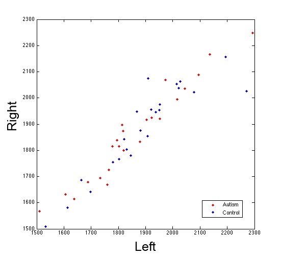
Figure 1-1. The left and right
amygdale volume for all subjects published in Chung et al. (2010)
[6]. There is no group difference and no hemisphere
difference.
4. Amygdala Surface
Flattening
January 20,
2008
The surface
flattening from an amygdala surface to a unit sphere is
needed for establishing a spherical harmonic parameterization on
the amygdala surface [1] [6]. We have developed a novel
flattening techniue using heat diffusion. We first enclose the
amygdala binary mask with a larger sphere (Figure 2 left). Take the
amygadala as a source (value +1) and the sphere as a sink (value
-1).
[amyg,sphere,amygsphere]=CREATEenclosedamyg(vol,surf);
figure;imagesc(squeeze(amygsphere(:,25,:)));colorbar
With the heat sink and source, we perform isotropic
heat diffusion for long time. After suffiient amount of
time, we reach a stady state, which is equivalent to solving the
Laplace
quation. The following code will run approximately 1
min. per surface in a qaud-core computer. The
result is given in Figure 2.
The last arguemnt indicates the number of iterations used to
obtain the steady state heat equation. In publication [6], 30
iterations were used but for simple shape like amygdala, 5
iterations are probably sufficient.
stream=LAPLACE3Dsmooth(amygsphere,amyg,-sphere,5);
figure;imagesc(squeeze(stream(:,25,:)));colorbar
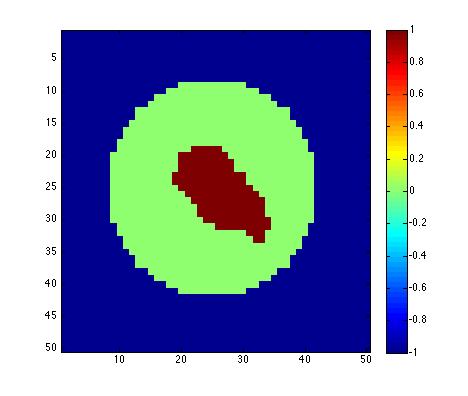

Figure 2. Left:
The amygdala is asigned the value 1 and the sphere enclosing
the amydala is asigned the value -1. Right: After solving
isotropic heat diffusion for long time, we reach a statedy
state, which can be used to generate a mapping from the
amygdala surface to the sphere by taking the geodesic path
from value 1 to -1.
The
stady state map (Figure 2)
is used to generate a mapping from the amygdala surface to the
sphere. This is done by computing the geodesic path from the
source to the sink. We first compute the levet sets of the
stady state corresponding to f(p) = c for -1 <= c <=1 and
propagate the amygdala boundary (c=1.0 in Figure 3) to the next level
set (c=0.6) by computing the geodesic path. The propagation from
one level set to the next is done by LAPLACEcontour.
The flattening process is expected to produce discretization
error. For each level set, we regularize mesh by shrinking down
larger than expected area of triangles using REGULARIZEarea.
20% of the larger than expected triangles are reduced in size by
setting the parameter to 0.8 in REGULARIZEarea.
sphere=isosurface(amyg);
for
alpha=1:5
sphere=LAPLACEcontour(stream,sphere,
1
- 2*alpha/5);
sphere=REGULARIZEarea(sphere,
0.8);
figure_wire(sphere,'yellow')
end;
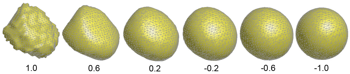
Figure 3. Amygdala surface flattening process
using the geodesic path of of the stady state map. The
parameters correspond to the level set f(p)=1.0, 0.6, ..., -0.6,
-1.0.
5. Weighted Spherical
Harmonic Representation (SPHARM)
January 22,
2008
Once we establish the mapping
from the amygdala surface onto a sphere, we can determine the spherical
angles \theta and \varphi. The domain of \theta
and \varphi in this study follows the convention established in
[1][2][3][6], which is different from the result directly
obtained from the built-in MATLAB function cart2sph.m.
Continuing directly from the above for-end loop, we run
[theta varphi]=EULERangles(surf);
surf=isosurface(amyg);
figure_trimesh(surf,theta)
figure_trimesh(surf,varphi)
figure_trimesh
projects Euler angles \theta and \varphi to the amygdala surface
(Figure 4). The
spherical angles are necessary to establish the weighted
spherical harmonic representation on a unit sphere. The
additional MATLAB implementation details on the weighted
spherical harmonic representation can be found in this link [click
here].
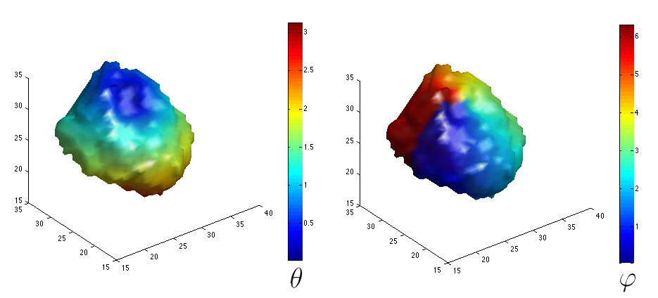
Figure 4. The spherical
angles projected onto an amygdala surface. North pole is taken
where \theta=0 (blue peak in the left figure).
The weighted spherical harmonic
representation of degree 60 and bandwidth sigma=0 is given by
running the code
[surf_smooth,
fourier]=SPHARMsmooth2(surf,sphere,60,0);
figure_wire(surf_smooth,'yellow')
where surf is the amygdala
surface and sphere is the spherical mesh
obtained by running LAPLACEcontour
and REGULARIZEarea. When the bandwidth is
zero, i.e. sigma=0, the weighted spherical harmonic
representation becomes the traditional spherical harmonic
representation. See refernce [2] and [3] for detail. Figure 5 shows various
degree representation.
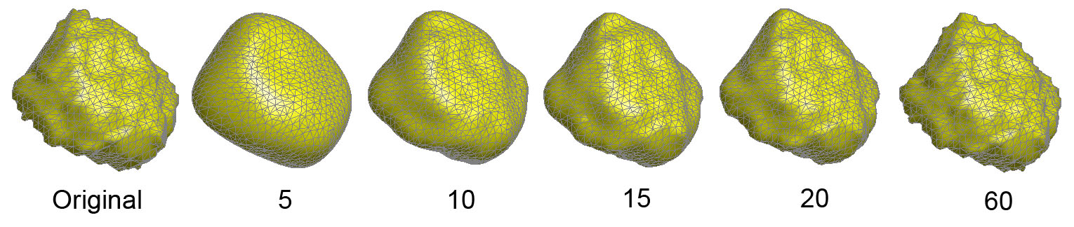
Figure 5. Spherical harmonic representations of
an amygdala surface.
The Fourier
series are known to introduce the Gibbs phenomeon
(ringing artifacts) [1]. The Gibbs phoenomeon occurs near
rapidgly changing or discontinous measurments. Since the
spherical harmonics are continuous and smooth basis functions,
it is not possible to represent discontinuity of data using
spherical harmonics.

Figure 6. The Gibbs
phenomeon is particuarly visible in the SPHARM representation
with k=42 and sigma=0. The ringing artifact is reduced if we
introduce a bit of smoothing sigma=0.001.
6. Saving and Loading
Multiple Surfaces
January
30, 2008
The following line of codes will process a
surface corresponding to subject id(i,:) and save the results
into a seperate *.mat file.
for i=1:size(id,1)
%put surface flattening + weighted
spherical harmonic modeling here
id_write=strcat('study1.right.',id(i,:),'.mat');
save(id_write,'fourier');
end
We
can load *.mat files iteratively and save them into a
structrued array study1_left:
for i=1:size(id,1)
file_name=strcat('study1.left.',id1(i,:),'.mat');
load(file_name);
study_left(i,:)=fourier;
end;
The Fourier coefficinets of the
10th-subject is given by
>
study_left(10,:)
ans =
x: [43x85 double]
y: [43x85 double]
z: [43x85 double]
7. Constructing
Average Amygdala Surface Template
January
30, 2008; March 29, 2008
The average
amygdala surfaces are constructed by averaging the collection
of Fourier coefficients up to degree 15. unitsphere2562.mat
is a spherical mesh with 2562 vertices. This is the mesh
resolution we will resample the average amygdala surface.
load unitsphere2562.mat
left_average=SPHARMaverage(study_left,sphere,
15,0.01);
figure_patch(left_average,'yellow');
right_average=SPHARMaverage(study_right,sphere,
15,0.01);
figure_patch(right_average,'yellow');
To construct
average surface template with only control subjects, modify
the above code to
left_average=SPHARMaverage(study_left(~group),sphere,
15,0.01);
The parameter
sigma=0.01 introduce a bit of smoothness into the
representation [1].

Figure 7. The average left
and right amygdala surfaces over 47 subjects (24 control and 23
autistic subjects).
8. Hotelling's
T-square Test for Two Samples
January 30,
2008
From
study_left and study_right that contain Fourier coefficients, we
construct the weighted spherical harmonics with degree 15
and bandwidth sigma 0.01. The resulting coordinates are
stored as matrices left_surf and right_surf.
left_surf=zeros(2562,3,47);
right_surf=zeros(2562,3,47);
for
i=1:47
temp=SPHARMrepresent2(sphere,study_left(i),15,0.01);
left_surf(:,:,i)=temp.vertices;
temp=SPHARMrepresent2(sphere,study_right(i),15,0.01);
right_surf(:,:,i)=temp.vertices;
end;
left_c=left_surf(:,:,find(~group));
left_a=left_surf(:,:,find(group));
right_c=right_surf(:,:,find(~group));
right_a=right_surf(:,:,find(group));
left_c
contails all surface coordinates for control subjects while
left_a contains all surface coordinates for autistic subjects. Then the Hotelling's T-square statistic is
used to measure the discrepancy between autistic and control
amygdala surfaces.
[h
p]=hotelT2(left_c,left_a);
h is the
Hotelling's T-square statistic and p is the corresponding
p-value (uncorrected).
figure_hotelT2(left_c,left_a,0.1,sphere);

Figure 8. The p-value of testing the
significance of group difference projected on to the mean
control surface. The white arrows indicate where to move the the
mean control surface to match it to the mean autistic surface. The
Hotelling's T-square did not detect significant difference (at
the corrected p-value of 0.05) although there is a huge cluster
on the right amygdala.
9. Multivariate
General Linear Model (MGLM) Using SurfStat
April 25,
2008
The problem with the Hotelling's T-square approach is the lack
of control for other covariates such as the global brain size
and age. So we need to covriate these nuisance variables
into a statistical model. This can be done if we use the multivarite
general linear models (MGLM) framework, which is implmented in Keith
Worsley's SurfStat
package [6]. In order to peform the
analysis given here, you need to download the package,
install it and set up the proper path.
Suppose we load age, brain size and group variables
(0=control, 1=autism) as
>>
age
age =...
15
18
15
>>brain
brain
=...
1.0091
1.1139
1.2173
>>
group
group
=...
0
0
1
Suppose we performed the
weighted-SPHARM and obtained the spherical harmonic coefficients
up to degree 40 for all 22 subjects. The results is saved in *.mat
file. The following codes display the coefficients of the
x-cooridinates of the left amygdala of the 1st subject.
load
amygdala.fourier.mat
x=fourier_left(1).x;
imagesc(x); colorbar
SurfStat needs to rearrange the array
of coordinates as 22 (number of surfaces)*2562 (number of
vertices) * 3 (dimension).
leftsurf=zeros(22,
2562,3);
rightsurf=zeros(22, 2562,3);
for i=1:22
temp=SPHARMrepresent2(sphere,fourier_left(i),40,0.001);
leftsurf(i,:,:)=temp.vertices;
temp=SPHARMrepresent2(sphere,fourier_right(i),40,0.001);
rightsurf(i,:,:)=temp.vertices;
end;
We need to convert our
average mesh to the SurfStat format.
avsurf.coord=right_average.vertices'
avsurf.tri=right_average.faces';
Then we obtain the displacement between each surface to the
average surface.
avg=kron(left_average.vertices,ones(46,1));
avg=reshape(avg,46,2562,3);
disp=left_surf-
avg;
The displacement vector field is used as a response variable in
the GLM. Using SurfStat codes, we define terms.
Age=term(age);
Group=term(group);
Brain=term(brain);
This amazing function enable us to set up a MGLM exactly like
in R/Splus. To test the group effect while controlling for
brain size and age, we set up a reduced and a full models,
and compute the ratio of sum of squared resiauls as
slm0 =
SurfStatLinMod( disp, Brain + Age + Group,avsurf);
slm = SurfStatT(slm0, group);
figure_trimesh(left_average,slm.t)
The T-statistic value is stored in slm.t. To
compute the random field theory based threshoding for given
P-value, run
>pvalue = [0.001 0.005 0.01 0.05 0.1]
>threshold=randomfield_threshold(slm,
pvalue)
pvalue =
0.0010
0.0050 0.0100
0.0500 0.1000
threshold =
6.8058
6.2154 5.9564
5.3398 5.0635
The
T-stat threshold of 4.7354 corresponds to the corrected P-value of
0.05.

Figure
9. The maximum T-stat (left) is 3.7970 but it will not
pass the random field theory based multiple comparision
thresholding at 0.05 level (5.3398).
10. Brain and Behavior
Correlation
May 8, 2008
Nacewicz et al. [3] showed that the smaller
amygdala volume predicts the smaller gaze fixation duration (eye
over face) in autism: individual with smaller amygdale showed the
least fixation of eyes relative to other facial regions. We wanted
to test if the local anatomical difference in amygdala is
correlated with the gaze fixation duration (Figure 10).
fixation=eye./face
fa=
fixation(find(group))
fc=fixation(find(~group))
[mean(fa)
std(fa)]
[mean(fc)
std(fc)]
[h,p] =
ttest2(fa,fc)
Fixation=term(fixation);
slm0 =
SurfStatLinMod( rightsurf, Brain + Age + Group +Fixation);
slm1 =
SurfStatLinMod( rightsurf, Brain + Age + Group + Fixation +
Group*Fixation, leftavsurf);
slmF =
SurfStatF(slm1, slm0);
figure_orgami(left_average,slmF.t)
resels =
SurfStatResels(slmF)
stat_threshold(
resels, length(slmF.t), 1, slm.df, 0.05, [], [], [], slmF.k )
temp=slmF.t;
temp(find(temp>40))=40;
figure_orgami(right_average,temp)

Figure
10. Significant interaction difference betewen the group
variable and the gaze fixation duration for the left (a) and right
(b) amygdale. See Chung et al. 2010 [6] for detail.
References
January 6, 2008;
October 15, 2011
- Chung, M.K. Nacewicz, B.M., Wang, S., Dalton,
K.M., Pollak, S., Davidson, R.J. 2008. Amydala
surface
modeling with weighted spherical harmonics. 4th
International Workshop on Medical Imaging and Augmented
Reality (MIAR). Lecture Notes in Computer Science (LNCS)
5128:177-184.
- Chung, M.K., Dalton, K.M., Davidson, R.J. 2008. Tensor-based
cortical
surface morphometry via weighed spherical harmonic
representation. IEEE Transactions on Medical Imaging.
27:1143-1151.
- Chung, M.K., Dalton, K.M., Shen, L., L., Evans,
A.C., Davidson, R.J. 2007. Weighted
Fourier
series representation and its application to quantifying the
amount of gray matter. Special Issue of IEEE
Transactions on Medical Imaging, on Computational
Neuroanatomy. 26:566-581.
- Nacewicz, B.M. and Dalton, K.M. and Johnstone,
T. and Long, M.T. and McAuliff, E.M. and Oakes, T.R. and
Alexander, A.L and Davidson, R.J. 2006. Amygdala volume and
nonverbal social impairment in adolescent and adult males with
autism. Arch. Gen. Psychiatry. 63:1417-1428
- Chung, M.K.,Qiu, A., Nacewicz, B.M., Dalton,
K.M., Pollak, S., Davidson, R.J. 2008. Tiling
manifolds
with orthonormal basis. 2nd MICCAI Workshop on
Mathematical Foundations of Computational Anatomy (MFCA).
- Chung, M.K., Worsley, K.J., Nacewicz, B.M.,
Dalton, K.M., Davidson, R.J. 2010. General
multivariate linear modeling of surface shapes using
SurfStat. NeuroImage. 53:491-505.