Estimator
-
$\hat{\beta}_{IV} = (Z'X)^{-1}Z'T$ is consistent whereas
$\hat{\beta}_{OLS} \mbox{ is not}$
-
Interpretation as Two-stage least squares:
-
$\hat{\beta}_{2SLS} = (\hat{X}'\hat{X})^{-1}\hat{X}'T \mbox{, where } \hat{X} = Z(Z'Z)^{-1}Z'X$
is another consistent IV estimator
-
Equivalent to regressing $X \mbox{ on } Z$ and then regressing $T \mbox{ on } \hat{X}$ from the first regression
Instrumental Variables in Survival Analysis
- Challenges
-
Traditional IV methods require linearity
-
Parametric models are often too restrictive for survival data in medical settings
-
Methods that do not require linearity typically require other strong assumptions,
such as no measurement error for the endogenous variable $X$
- Some assumptions must be made
-
In a completely nonparametric model, there are identifiability issues
Instrumental Variables in Survival Analysis
-
Existing work for IV methods for survival data
-
Most work relies on fully specified parametric structural equation models:
Tang and Lee (1998), Muthen and Masyn (2005), and Chen, et al (2011)
-
Two-stage residual inclusion (Terza et al., 2008)
allows for consistent estimation for nonlinear parametric models with no censoring
-
Recent has moved away from parametric outcome models, incorporating instrumental variable estimation in the Cox proportional hazards model (MacKenzie et al., 2014) and the additive hazards model (Li et al., 2015; Tchetgen Tchetgen et al., 2015)
which alleviates some of the restrictions of fully parametric approaches
-
However, they all impose a structural model for the confounding mechanism or parametric assumptions on the IV model
Review: Accelerated Failure Time Model
-
$\log \widetilde{T}_i = \beta X_i + \epsilon_i$, $i=1,\dots,n \mbox{ where }\epsilon_i$ come from a common, unspecified distribution and $\epsilon_i \perp\!\!\!\perp (X_i, C_i)$
Let $C_i$ be the censoring time for subject $i$, where $C_i \perp\!\!\!\perp \widetilde{T}_i | X_i$
We observe $(T_i, \Delta_i, X_i), \mbox{ where } T_i = \widetilde{T}_i \wedge C_i \mbox{ and } \Delta_i = I(\widetilde{T}_i \leq C_i) $
- Nice interpretation: $\log$ of the survival time is linear in the covariates
- Linearity provides opportunity for use of IVs
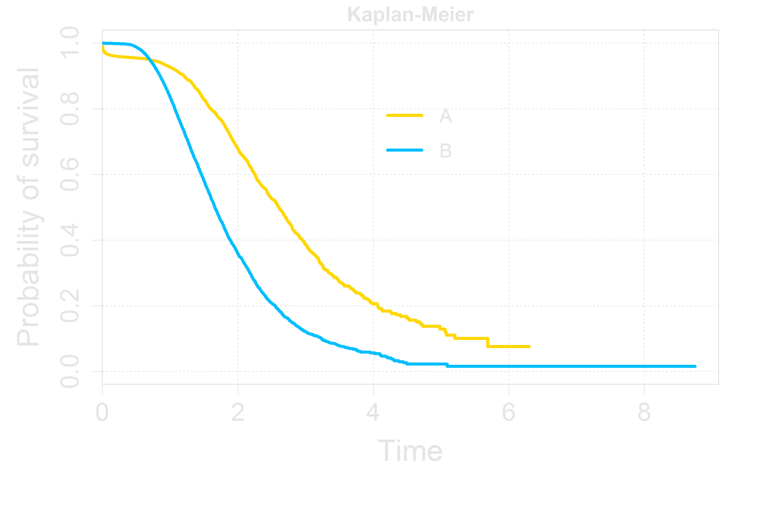
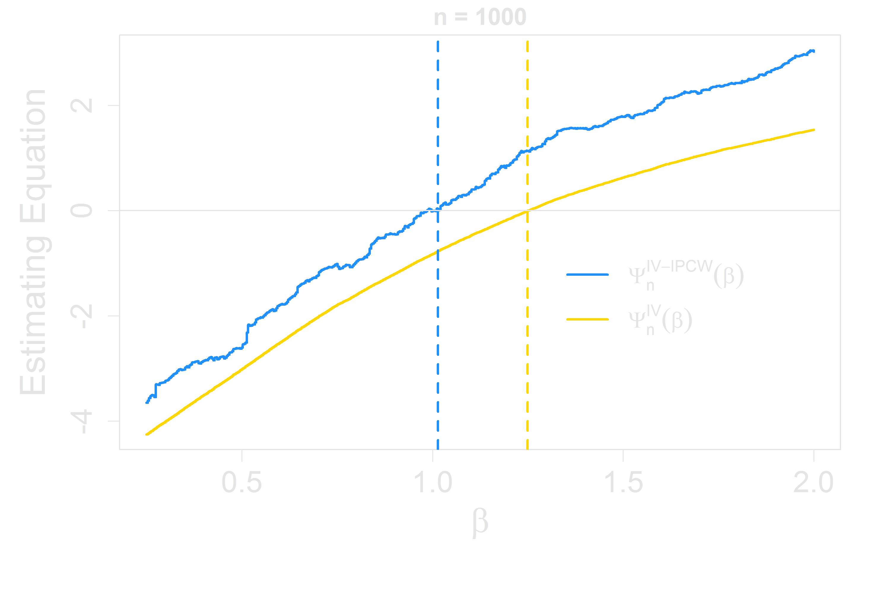
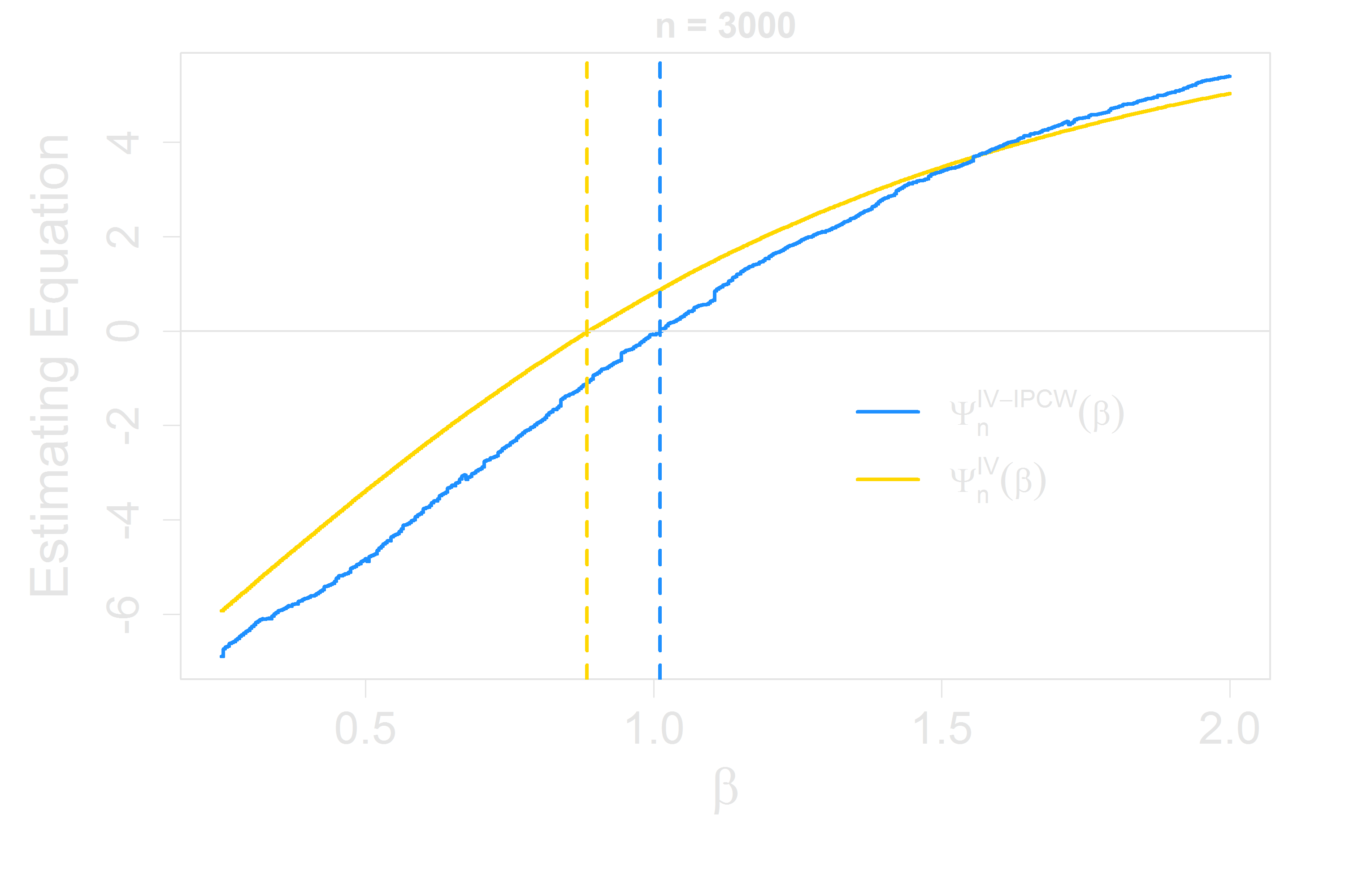
Simulation from log-normal AFT Model with Crossing
Review: AFT Model Estimation
Rank-based Estimation of $\beta$
\begin{align*}
\Psi_n(\beta) &= \sum_{i = 1}^n\int \rho(t, \beta)\{ X_i - \overline{X}(t, \beta) \} \mbox{ } \mathrm{d}N_i(t; \beta) \\
& \\
\mbox{where } \overline{X}(t, \beta) &\equiv
\frac{1}{n}\sum_{j=1}^n X_j I(\epsilon_j^\beta \ge t) \mbox{ } / \mbox{ } \frac{1}{n}\sum_{j=1}^n I(\epsilon_j^\beta \ge t) \mbox{ and} \\
& \\
\epsilon_i^\beta &= \log{T_i} - \beta X_i \mbox{ is the residual for subject }i \\
\mbox{ and }
N_i(t; \beta) &= I(\epsilon_i^\beta \leq t, \Delta_i = 1)
\end{align*}
$\hat{\beta}$ is the zero crossing of $\Psi_n(\beta)$.
Its asymptotic normality was proved by Tsiatis (1990) and Ying (1993)
Review: AFT Model Estimation
Rank-based Estimation of $\beta$
\begin{align*}
\Psi_n(\beta) &= \sum_{i = 1}^n\int \rho(t, \beta)\{ X_i - \overline{X}(t, \beta) \} \mbox{ } \mathrm{d}N_i(t; \beta) \\
&
\end{align*}
- Computational Challenges
-
$\Psi_n(\beta)$ is neither continuous nor monotone
-
Continuous approximations to $\Psi_n(\beta)$
-
To ensure monotonicity, let $\rho(t, \beta) = \frac{1}{n}\sum_{j=1}^n I(\epsilon_j^\beta \ge t)$ (Gehan weighting)
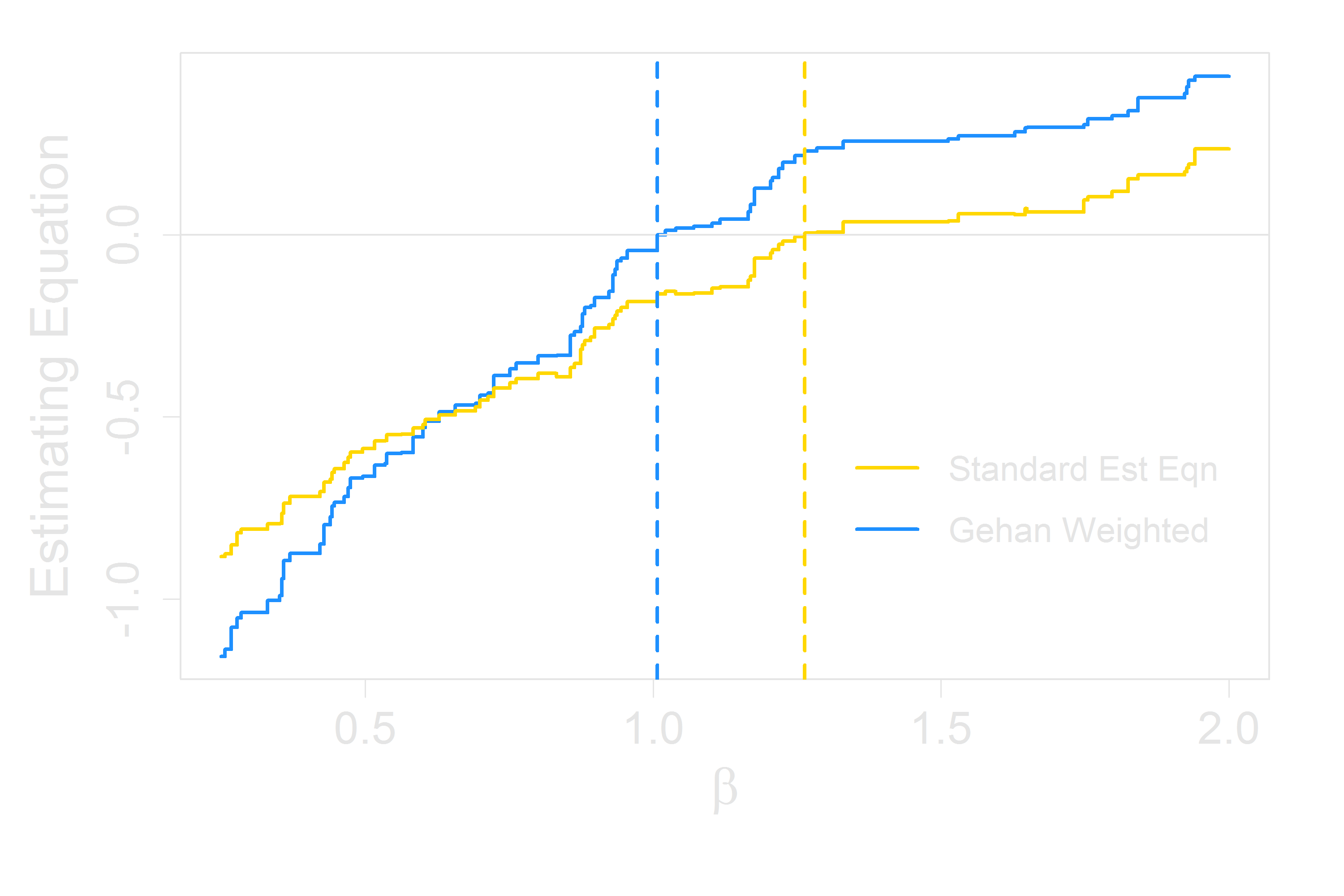
AFT Estimating Equation
Assumptions for IVs in the Accelerated Failure Time Model
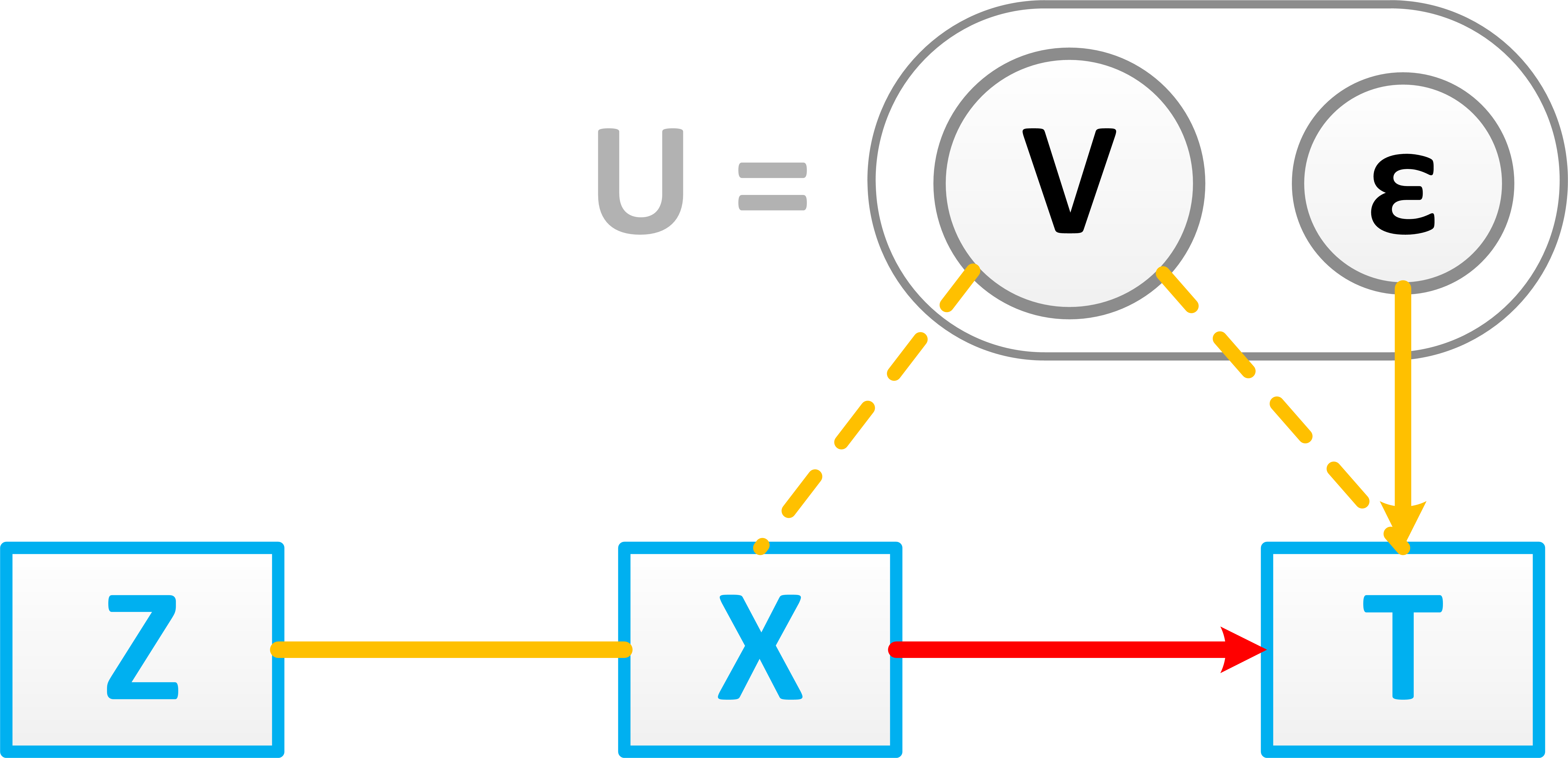
- The underlying model is:
$\log \widetilde{T}_i = \beta X_i + U_i$,
$i=1,\dots,n$
- where
-
$Z_i\perp\!\!\!\perp U_i$
-
$\widetilde{T}_i\perp\!\!\!\perp Z_i|X_i, U_i$
-
$X_i \not\!\perp\!\!\!\perp Z_i$
-
A key difference from standard AFT assumptions:
-
$C_i\perp\!\!\!\perp (X_i, Z_i, U_i, \widetilde{T}_i)$
Methods for Unmeasured Confounders - possible estimator of $\beta$
In the spirit of 2SLS, replace $X$ with ${\color{Yellow}\hat{X}} = Z(Z'Z)^{-1}Z'X$
\begin{align*}
\Psi_n^{2SLS}(\beta) &= \sum_{i = 1}^n\int \rho(t, \beta)\{ {\color{Yellow}\hat{X}_i} - {\color{Yellow}{\tilde{X}}(t, \beta)} \} \mbox{ } \mathrm{d}N_i(t; \beta) \\
& \\
\mbox{where } {\color{Yellow}{\tilde{X}}(t, \beta)} &\equiv
\frac{1}{n}\sum_{j=1}^n {\color{Yellow}\hat{X}_j} I({\color{Yellow}\hat{\epsilon}_j^\beta} \ge t) \mbox{ } / \mbox{ } \frac{1}{n}\sum_{j=1}^n I( {\color{Yellow}\hat{\epsilon}_j^\beta} \ge t) \mbox{ and} \\
& \\
{\color{Yellow}\hat{\epsilon}_i^\beta} &= \log{T_i} - \beta {\color{Yellow}\hat{X}_i} \mbox{ is the residual for subject }i \mbox{ and }
N_i(t; \beta) = I({\color{Yellow}\hat{\epsilon}_i^\beta} \leq t, \Delta_i = 1)
\end{align*}
However this still imposes a linear
assumption on the effect of the IV on $X$
Methods for Unmeasured Confounders - possible estimator of $\beta$
In the spirit of IV, replace $X$ with ${\color{Yellow}Z}$
\begin{align*}
\Psi_n^{IV}(\beta) &= \sum_{i = 1}^n\int \rho(t, \beta)\{ {\color{Yellow}Z_i} - {\color{Yellow}\overline{Z}(t, \beta)} \} \mbox{ } \mathrm{d}N_i(t; \beta) \\
& \\
\mbox{where } {\color{Yellow}\overline{Z}(t, \beta)} &\equiv
\frac{1}{n}\sum_{j=1}^n {\color{Yellow}Z_j} I(\epsilon_j^\beta \ge t) \mbox{ } / \mbox{ } \frac{1}{n}\sum_{j=1}^n I(\epsilon_j^\beta \ge t) \mbox{ and} \\
& \\
\epsilon_i^\beta &= \log{T_i} - \beta {\color{Yellow}X_i} \mbox{ is the residual for subject }i \mbox{ and }
N_i(t; \beta) = I(\epsilon_i^\beta \leq t, \Delta_i = 1)
\end{align*}
We compare ${\color{Yellow}Z_i} \mbox{ with } {\color{Yellow}\overline{Z}(t, \beta)}$,
the mean IV value for those in the risk set for $i$
Methods for Unmeasured Confounders - possible estimator of $\beta$
However, in
\begin{align*}
\Psi_n^{IV}(\beta) &= \sum_{i = 1}^n\int \rho(t, \beta)\{ {\color{Yellow}Z_i} - {\color{Yellow}\overline{Z}(t, \beta)} \} \mbox{ } \mathrm{d}N_i(t; \beta) \\
& \mbox{ } \\
\epsilon_i^\beta &= \log{T_i} - \beta {\color{Yellow}X_i} \mbox{ depends on } {\color{Yellow} C_i}
\end{align*}
and thus this estimator is not consistent for $\beta$
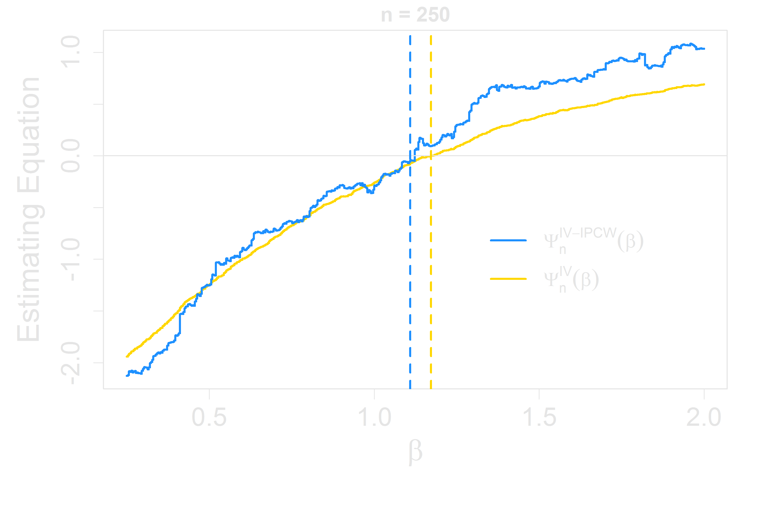
IV Estimation in the Accelerated Failure Time Model
A natural method for handling non-ignorability of censoring is inverse probability-of-censoring weighting
\begin{align*}
\Psi_n^{IV-IPCW}(\beta) &= \sum_{i = 1}^n\int \rho(t, \beta)\{ {\color{Yellow}Z_i} - {\color{Yellow}\overline{Z}_{\hat{G}_C}(t, \beta)} \} \frac{\mathrm{d}N_i(t; \beta)}{\hat{G}_C(t + \beta X_i)} \\
& \\
\mbox{where } {\color{Yellow}\overline{Z}_{\hat{G}_C}(t, \beta)} &\equiv
\frac{1}{n}\sum_{j=1}^n \frac{{\color{Yellow}Z_j} I({\color{Yellow}\epsilon_j^\beta} \ge t)}{\hat{G}_C(t + \beta X_j)} \mbox{ } / \mbox{ }
\frac{1}{n}\sum_{j=1}^n \frac{I( {\color{Yellow}\epsilon_j^\beta} \ge t)}{\hat{G}_C(t + \beta X_j)} \mbox{ and} \\
& \\
{\color{Yellow}\epsilon_i^\beta} &= \log{T_i} - \beta {\color{Yellow}X_i} \mbox{ is the residual for subject }i \\
\mbox{ and }
N_i(t; \beta) &= I({\color{Yellow}\epsilon_i^\beta} \leq t, \Delta_i = 1)\\
\mbox{and } \hat{G}_C & \mbox{ is the Kaplan-Meier estimator of } G_C\mbox{, the survival function of } C
\end{align*}
Asymptotic Theory for IVs in the Accelerated Failure Time Model
Theorem 1
Assume regularity conditions hold and ${\rho}_n(t, \beta)$ and $\overline{Z}_{\hat{G}_C}(t, \beta)$ in $\Psi_n^{IV-IPCW}(\beta)$ belong to Glivenko-Cantelli classes. Then an approximate root $\hat{\beta}_n$ satisfying
\begin{align*}
\Psi_n^{IV-IPCW}({\hat{\beta}_n}) = o_{p*}(1)
\end{align*}
is consistent. In particular when ${\rho}_{\hat{G}_C, n}(t,\beta) = \frac{1}{n}\sum_{i=1}^n \frac{I( {\epsilon_i^\beta} \ge t)}{\hat{G}_C(t + \beta X_j)}$ for the Gehan type of weight, the resulting estimator is consistent.
Asymptotic Theory for IVs in the Accelerated Failure Time Model
Theorem 2
Denote $\hat{\gamma}_n = \hat{G}_C^{-1} \mbox{, } \gamma_0 = G_C^{-1}$ and let $\hat{\beta}_n$ be an approximate
root satisfying
\begin{align*}
\Psi_{\hat{\gamma}_n, n}^{IV-IPCW}(\hat{\beta}_n) = o_{p^*}(n^{-1/2}).
\end{align*}
Then under the regularity conditions, $n^{1/2}(\hat{\beta}_n - \beta_0)$ is asymptotically normal with the
asymptotic representation
\begin{align*}
n^{1/2}( \hat{\beta}_n - \beta_0 ) = n^{1/2}( \widetilde{\beta}_n - \beta_0 ) - \{ \dot{\Psi}_\beta (\beta_0) \}^{-1} \dot{\Psi}_{\gamma} ( n^{1/2} (\hat{\gamma}_n - \gamma_0) ) + o_{p^*}(1)
\end{align*}
where $\widetilde{\beta}_n$ is an approximate root satisfying
\begin{align*}
\Psi_{\gamma_0, n}^{IV-IPCW}(\widetilde{\beta}_n) = o_{p^*}(n^{-1/2}).
\end{align*}
Computation for IVs in the Accelerated Failure Time Model
Computation for IVs in the Accelerated Failure Time Model
Computation for IVs in the Accelerated Failure Time Model
Computation for IVs in the Accelerated Failure Time Model
-
Utilization of the $\texttt{R}$ package $\texttt{BB}$
-
$\texttt{BB}$ is a derivative-free method for solving nonlinear systems of equations
-
Works well for non-smooth systems of equations
-
$\texttt{BB}$ doesn't always find the solution, so an adaptive restarting strategy is used, which makes solving more robust
Inference for IV Estimation in the AFT Model
-
Full bootstrap: solve $n^{-1/2}\Psi_n^{IV-IPCW^*}(\beta)$ $\mbox{ }B$ times, where
$n^{-1/2}\Psi_n^{IV-IPCW^*}(\beta)$
is the estimating equation based on resampled data
-
However, due to the computational difficulties in solving $n^{-1/2}\Psi_n^{IV-IPCW}(\beta)$,
this is impractical
-
Instead, if we can relate the variance of $n^{-1/2}\Psi_n^{IV-IPCW}(\beta)$ to the variance of
$n^{1/2}(\hat{\beta} - \beta_0)$, a greatly less computationally demanding procedure can be developed
-
This motivates the use of resampling strategies from Zeng and Lin (2008)
-
Instead of solving estimating equations, involves evaluating perturbed equations
-
Can accomodate nonsmooth estimating equations/functions
Standard AFT - Inference
-
For the standard AFT model, under some regularity conditions (Parzen et al. 1994, Zeng and Lin 2008):
-
Uniformly in a neighborhood of $\beta_0$,
$n^{-1/2}\Psi_n(\beta) = n^{-1/2}\sum_{i=1}^n S_i(\beta_0) + A n^{1/2}(\beta - \beta_0) + o_p(1+n^{1/2}||\beta - \beta_0||)$
where $A$ is the asymptotic slope of $\frac{1}{n}\Psi_n(\beta_0)$
-
Hence, $n^{1/2}(\hat{\beta} - \beta_0)$ is asymptotically norm with variance
$\Sigma = A^{-1}V(A^{-1})^T$, where $V = \lim_{n \to \infty}\frac{1}{n}\sum_{i=1}^nS_i S_i^T$
-
Zeng and Lin (2008) proposed to estimate $A$ by regressing the following perturbation
$n^{-1/2}\Psi_n(\hat{\beta} + n^{-1/2}Z_b),\mbox{ }Z_b \sim N(0,1)$ on $Z_b, b=1,\dots,B$ and to estimate
$V$ by taking the sample variance of $B$ resampled equations
$n^{-1/2}\Psi_n^{*}(\hat{\beta})$
Inference for IV Estimation in the AFT Model
- From Theorem 2 we have
\begin{align*}
n^{-1/2}\Psi_n^{IV-IPCW}(\beta) = {} & \dot{\Psi}_{\gamma} ( n^{1/2} (\hat{\gamma}_n - \gamma_0) ) + n^{-1/2}\sum_{i=1}^nS_i(\beta_0) \\
&{} +
An^{1/2}(\beta - \beta_0) + o_p(1 + n^{1/2}||\beta - \beta_0 ||) \\
\end{align*}
- And hence the bootstrap method applies
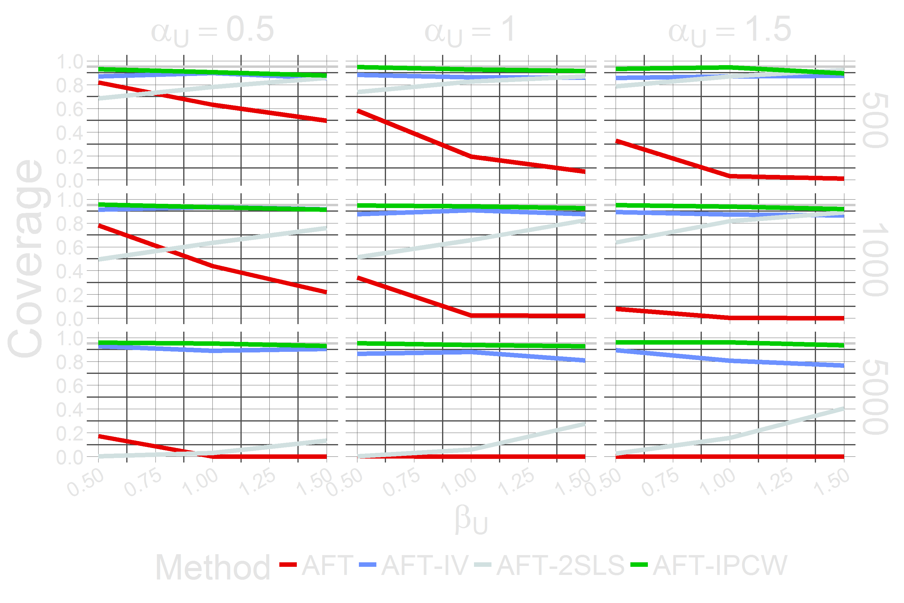
Simulation $\widetilde{T} = \exp{\{ \beta X + \beta_U U + \epsilon \}}$
where
$X = \alpha_Z \exp{\{Z\}} + \alpha_U U + \epsilon^* $ and
$\epsilon$, $\epsilon^* \sim N(0,1)$, $\epsilon \perp\!\!\!\perp \epsilon^*$
$\alpha_U = $
$Cor(U,X)=$
$\beta_U = $
$Cor(U,{T})=$
$\alpha_Z = $
$Cor(Z,X)=$
Coverage $\widetilde{T} = \exp{\{ \beta X + \beta_U U + \epsilon \}}$
where
$X = \alpha_Z \exp{\{Z\}} + \alpha_U U + \epsilon^* $
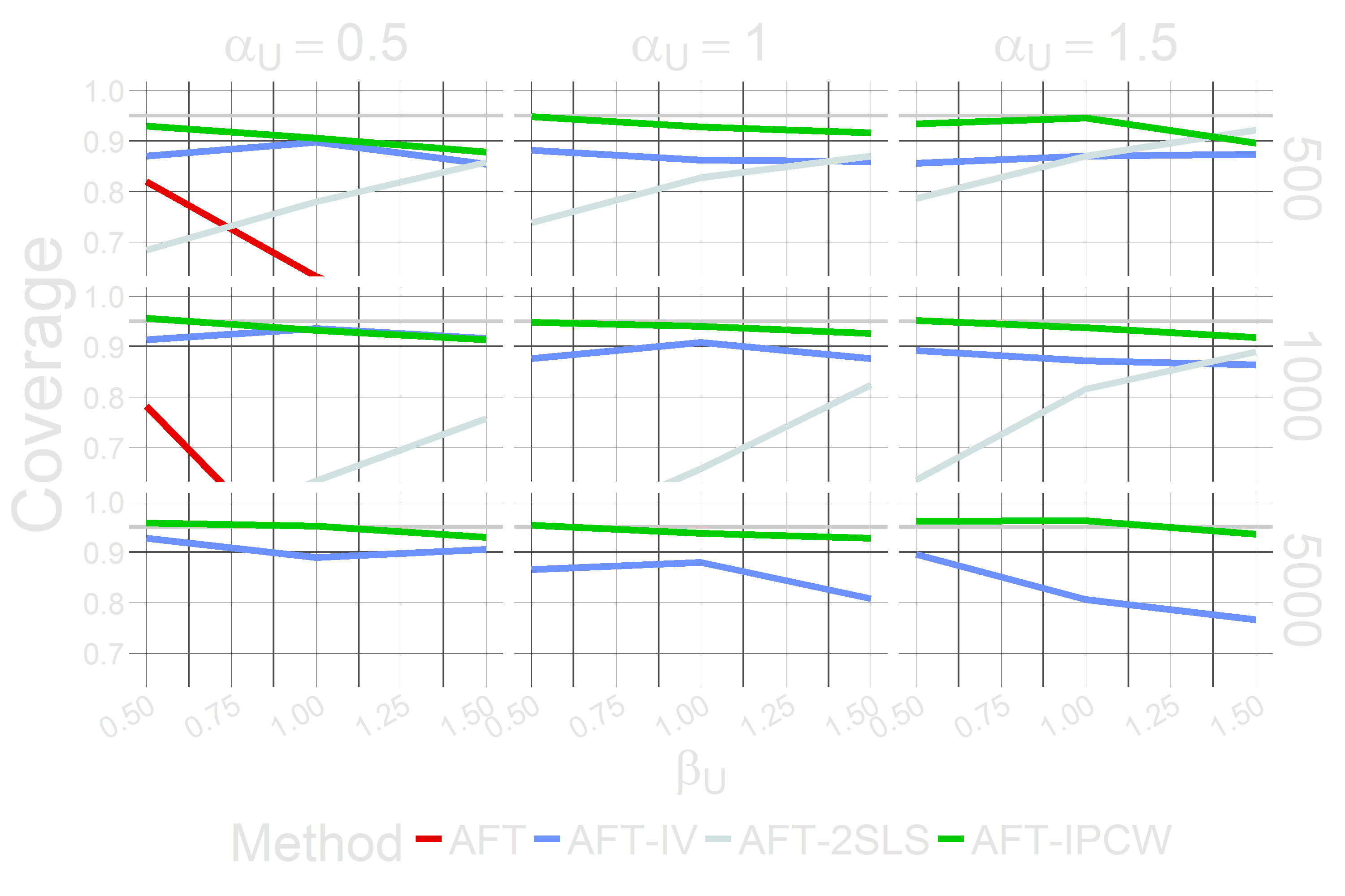
Coverage (Zooming In) $\widetilde{T} = \exp{\{ \beta X + \beta_U U + \epsilon \}}$
where
$X = \alpha_Z \exp{\{Z\}} + \alpha_U U + \epsilon^* $
Preliminary Analysis
-
Data
-
Rupture cases (2853 patients)
-
~66% censoring
-
9 years of follow-up
-
962 deaths, 733 of which were related to endo repair
-
Instrument: the proportion of endovascular AAA surgeries by institution in the past 365 days
-
Standard methods to determine instrument strength support the use of this as an instrument
- Methods
-
Standard AFT model, AFT model with IV replacement, AFT-2SLS, AFT-IV-IPCW
-
Bootstrap for confidence intervals
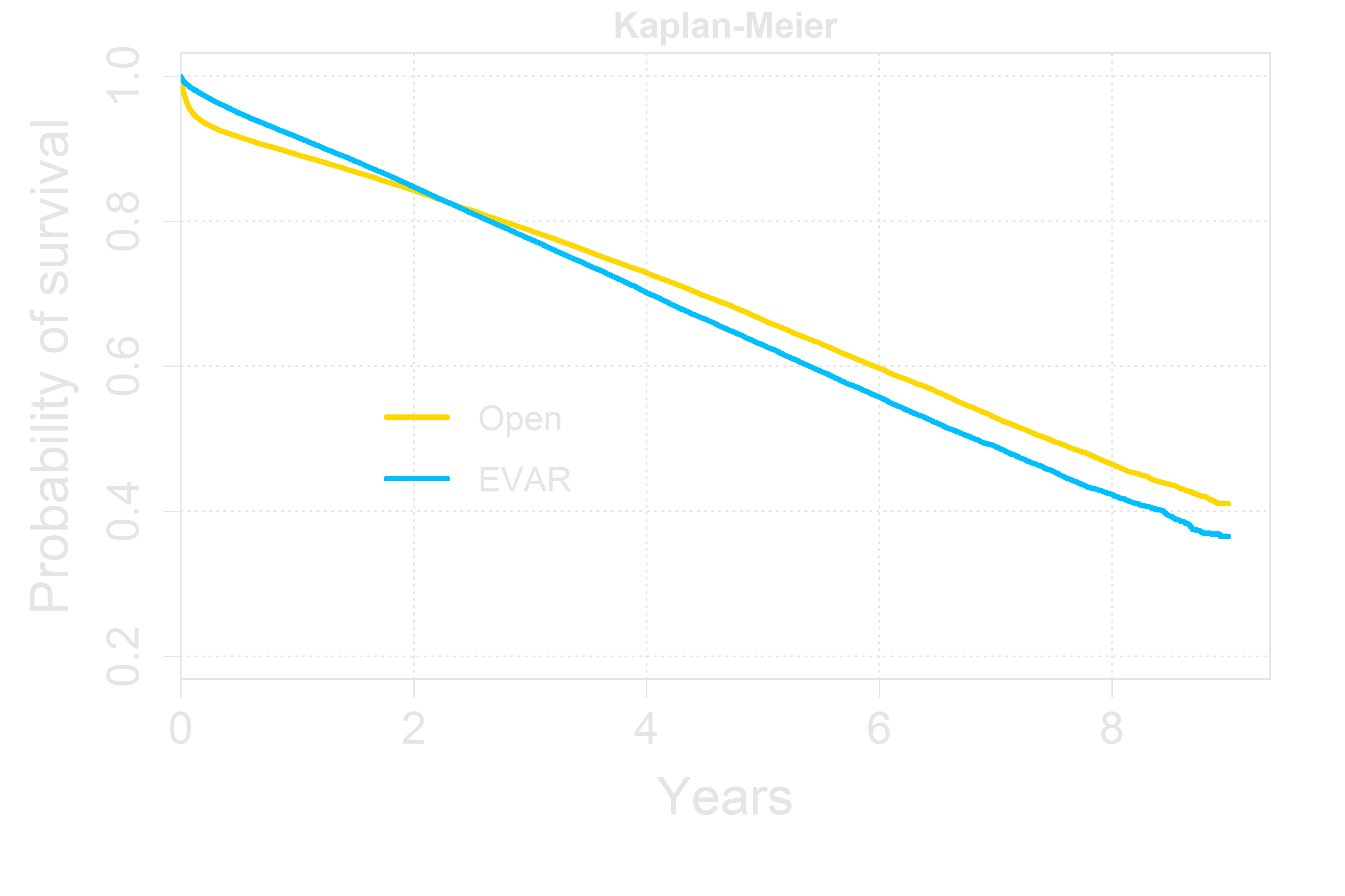
Kaplan-Meier Curves for All Patients
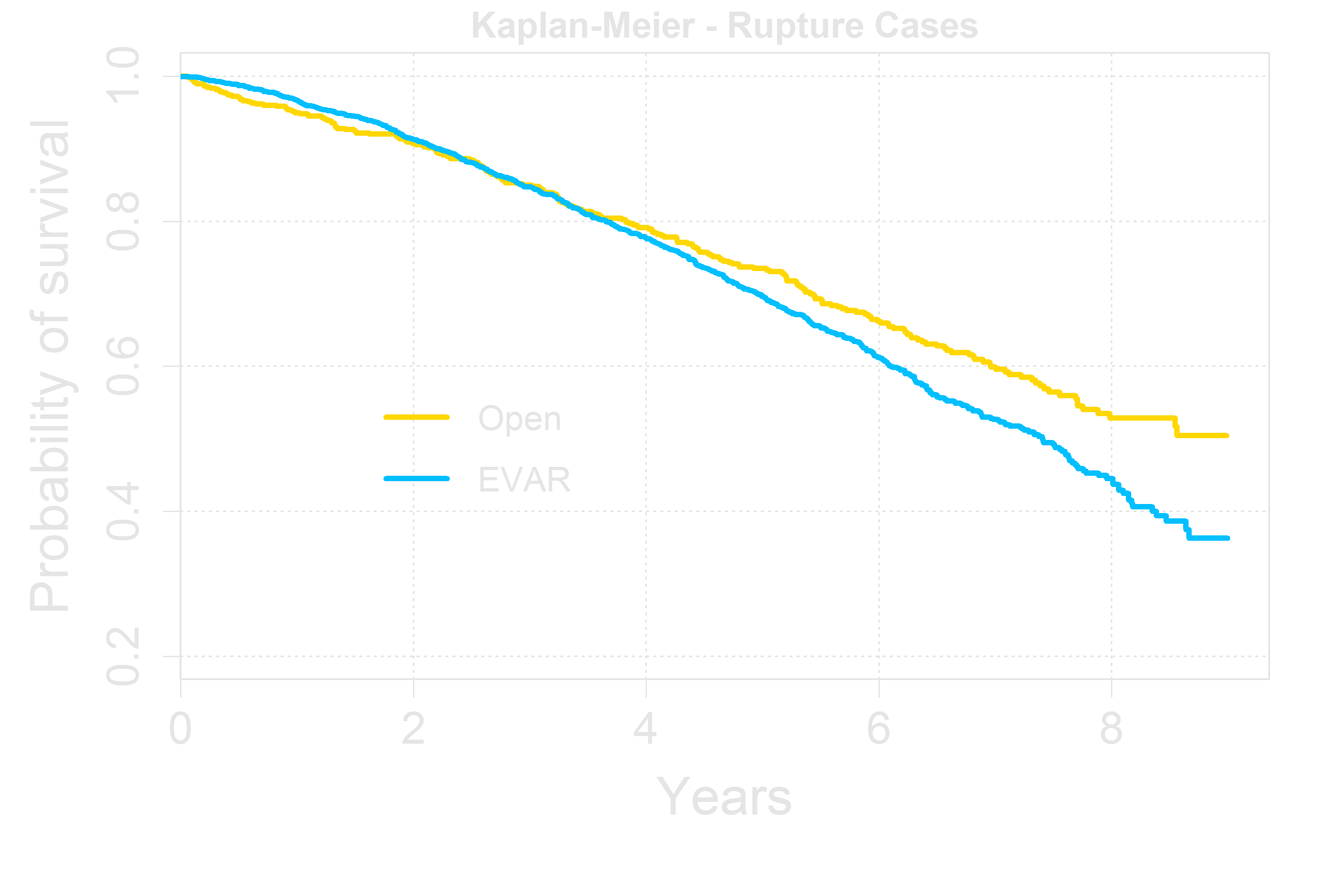
Kaplan-Meier Curves for Rupture Cases
Preliminary Analysis
Estimate of the effect of endovascular repair (EVAR)
on log survival time
accounting for prior conditions, demographic variables, and others
$
\begin{array}{c|rrl}
{\text{Estimator}} & {\hat{\boldsymbol\beta}_{EVAR}} & {(95\% \text{ Conf.}} & {\text{Interval})} \\
\hline
\text{AFT} & 0.047 & (-0.063, & 0.144) \\
\text{AFT-IV} & -0.169 & (-0.420, & 0.080) \\
\text{AFT-2SLS} & -0.175 & (-0.432, & 0.074) \\
\text{AFT-IV-IPCW} & -0.156 & (-0.364, & 0.052) \\
\end{array}
$
Conclusions
-
AAA Rupture Data
-
Standard AFT model (no IV adjustment) suggests slight benefit from endo
-
AFT-IV / 2SLS /IPCW models suggest potential benefit from open surgery
-
Interactions between the surgery type and patient characteristics
-
IV Estimation in the AFT model
- Standard AFT model exhibits clear bias in the presence of confounding
- AFT-IV is not consistent, but in practice is much better than AFT
- IPCW provides a theoretically sound IV method
←
→
/
