From flights to linear regression

Introduction to Multiple Regression

• Extends simple linear regression
• Predicts a dependent variable using multiple independent variables
• Each coefficient represents the relationship with the dependent variable, controlling for other variables

Review: Simple Linear Regression

• Dependent and independent variables
• The regression equation: \(Y = \beta_0 + \beta_1X_1 + \epsilon\)
• Fitting a line to data

From Simple to Multiple Regression

• Multiple regression equation: \(Y = \beta_0 + \beta_1X_1 + \beta_2X_2 + ... + \beta_nX_n + \epsilon\)
• “Controls for multiple variables simultaneously”

Multiple regression…

• Multiple regression equation: \(Y = \beta_0 + \beta_1X_1 + \beta_2X_2 + ... + \beta_nX_n + \epsilon\)
• What is the derivative \(\frac{d E(Y|X)}{d X_1}\)?
• In our data \(X_1\) and \(X_2\) are likely correlated… so what?

The Flights Dataset: A Recap

• Overview of dataset features relevant for regression
• Potential predictors: departure delay, distance, month, day of week

Preparing Data with dplyr

# Example of data preparation
my_flights = flights %>% 
  mutate(day_of_week = wday(time_hour)) %>%
  select(dep_delay, arr_delay, distance, month, day_of_week) %>% 
  filter(!is.na(dep_delay), !is.na(arr_delay))

Fitting a Multiple Regression Model

# Fitting the model
model <- lm(arr_delay ~ dep_delay + distance + month + day_of_week, data=my_flights)
summary(model)

Call:
lm(formula = arr_delay ~ dep_delay + distance + month + day_of_week, 
    data = my_flights)

Residuals:
     Min       1Q   Median       3Q      Max 
-107.713  -11.043   -1.974    8.699  205.871 

Coefficients:
              Estimate Std. Error t value Pr(>|t|)    
(Intercept) -2.585e+00  1.033e-01  -25.02   <2e-16 ***
dep_delay    1.018e+00  7.823e-04 1301.33   <2e-16 ***
distance    -2.550e-03  4.259e-05  -59.86   <2e-16 ***
month        2.259e-02  9.183e-03    2.46   0.0139 *  
day_of_week -1.980e-01  1.612e-02  -12.29   <2e-16 ***
---
Signif. codes:  0 '***' 0.001 '**' 0.01 '*' 0.05 '.' 0.1 ' ' 1

Residual standard error: 17.93 on 327341 degrees of freedom
Multiple R-squared:  0.8387,    Adjusted R-squared:  0.8387 
F-statistic: 4.255e+05 on 4 and 327341 DF,  p-value: < 2.2e-16

Interpreting Model Output

• Coefficients: Estimated effect of each predictor
• R-squared: Proportion of variance explained
• p-values: Statistical significance of predictors

Visualization

plot(model)

Model Diagnostics

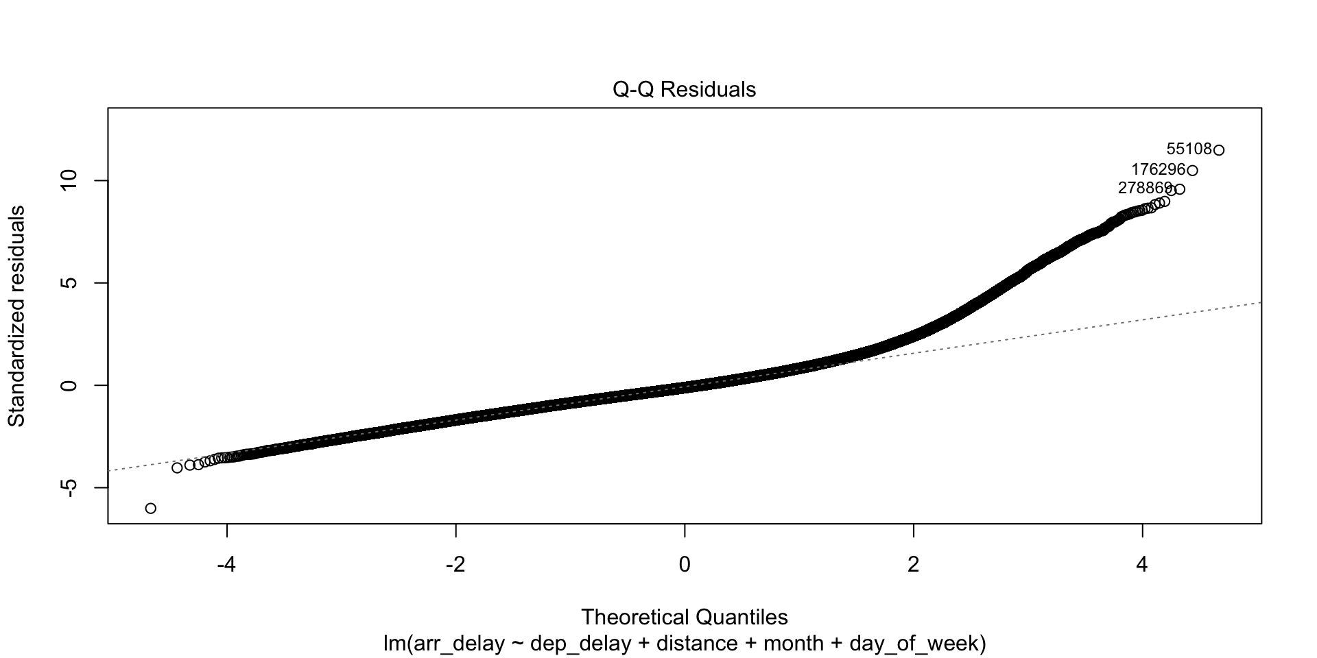
• Check for linearity, independence, homoscedasticity, and normality of residuals
• Importance of diagnostics in model evaluation

Multicollinearity: A Nuanced View

• Multicollinearity refers to high correlations among independent variables
• It can inflate standard errors and make coefficient estimates less reliable
• However, the presence of multicollinearity does not invalidate the model. It’s crucial for prediction, less so for inference where understanding individual predictors’ effects is important
• Removing variables solely based on multicollinearity should be approached with caution

Hands-On Exercises

• Modify models to include/exclude variables
• Interpret outputs

Conclusion and Further Learning

• Recap of multiple regression concepts
• Encourage further exploration and learning

Questions & Discussion

• Open floor for questions and sharing of experiences