|
Magnetic Resonance Image Segmentation with Thin Plate
Spline Thresholding
|
Xianhong Xie1,2, Moo K.
Chung1,2,3, Grace
Wahba1,2
1Department of Statistics, University
of Wisconsin-Madison, 2Department of Biostatistics and
Medical Informatics, University of Wisconsin-Madison, 3W.M. Keck Laboratory for Functional
Brain Imaging and Behavior, University of Wisconsin-Madison
|
Objective:
To develop a new
method for segmenting T1-Weighted magnetic resonance image
into gray matter (GM), white matter (WM), cerebrospinal fluid
(CSF), and other types of tissues.
Methods:
Our method has 4 steps. First, we divide each slice
into overlapping blocks. Second, we fit thin plate splines to
each block with different number of knots, and search for the
knots configuration that gives us the smallest GCV score with
a fudge factor [1].
Third, we fit the thin plate spline with the knots
configuration found, and predict on a really fine grid. We
also find the thresholds on the block with the K-means
algorithm. Finally, we blend the predicted block images and
the thresholds with some smooth weighting functions. The
averages of the corresponding thresholds on all the blocks and
the thresholds on the blended smooth image are calculated as
well. We can apply all 3 thresholding scheme to the blended
image, and pick the one that suits our needs best. Our
empirical results show that images from different sources
might need different thresholding.
The TPS method was
tested on 5 subjects from the IBSR 20 normal data. We selected
the 2nd, 6th, 10th, 14th, 18th subject after we sorted the 20
subjects based on their id's. One slice near the middle of the
brain for each subject was used with our method. SPM
segmentation was applied to the whole volumes of the 5
subjects. Note that the 20 normal data is provided with human
segmentation results.
Results & Discussion:
The comparison between TPS method, SPM, and manual
segmentation on one subject is given in Figure 1
and 2.
They show that TPS method matches manual segmentation
reasonably well. And the TPS is doing really close to SPM. The
correlation coefficients and kappa indices [2]
between each 2 of the 3 methods for all the subjects were
calculated (Table 1).
The numbers confirm our conclusions. Note that the TPS method
gives subpixel segmentation (Figure 3).
Conclusions:
Our method is an intensity based method. It uses thin
plate splines to reconstruct the image. Our results show that
the new method is comparable to the SPM segmentation, as well
as the human segmentation. The TPS method has the advantage of
giving subpixel level results and generating smoother
boundaries. The partial volume effects are addressed by the
subpixel segmentation. Also, it offers the potential for more
accurate estimate of distances and curvatures on the cortical
surfaces. Our method tackles the image non-uniformity through
local thresholding and blending. It depends less heavily on
correction for non-uniformity.
References &
Acknowledgements:
[1] Luo, Z. and Wahba,
G. (1997). Journal of the American Statistical Association,
92:107-116.
[2] Zijdenbos, A.P. et al
(1994). IEEE Transactions on Medical Imaging,
13:716-724.
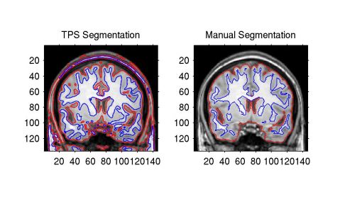
Figure 1: Comparison of TPS Segmentation vs
Manual Segmentation
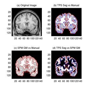
Figure 2: Pairwise Comparison of TPS, SPM,
and Manual Segmentation
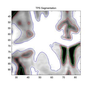
Figure 3: Zoomed View of the TPS
Segmentation Boundaries
| Table 1: Coefficients for all
the Comparisons with Mean and SD
Summary |
|
|
subject
no. |
corr. coef. |
kappa index |
| GM |
WM |
GM |
WM |
| tps vs
manual |
1 |
0.660 |
0.827 |
0.836 |
0.872 |
| 2 |
0.702 |
0.757 |
0.841 |
0.827 |
| 3 |
0.654 |
0.787 |
0.811 |
0.850 |
| 4 |
0.410 |
0.678 |
0.723 |
0.770 |
| 5 |
0.612 |
0.791 |
0.776 |
0.838 |
| mean(sd) |
|
0.608(0.115) |
0.768(0.056) |
0.798(0.049) |
0.831(0.038) |
| spm vs
manual |
1 |
0.675 |
0.846 |
0.883 |
0.866 |
| 2 |
0.686 |
0.839 |
0.887 |
0.880 |
| 3 |
0.637 |
0.810 |
0.863 |
0.842 |
| 4 |
0.091 |
0.672 |
0.679 |
0.753 |
| 5 |
0.450 |
0.803 |
0.825 |
0.824 |
| mean(sd) |
|
0.518(0.250) |
0.794(0.071) |
0.827(0.087) |
0.833(0.050) |
| tps vs spm |
1 |
0.806 |
0.883 |
0.848 |
0.900 |
| 2 |
0.626 |
0.759 |
0.794 |
0.824 |
| 3 |
0.734 |
0.822 |
0.808 |
0.861 |
| 4 |
0.426 |
0.767 |
0.730 |
0.793 |
| 5 |
0.645 |
0.800 |
0.785 |
0.836 |
| mean(sd) |
|
0.647(0.143) |
0.806(0.050) |
0.793(0.043) |
0.843(0.040) | |
|
|
|


